神经网络的数学推导公式

如题。

参考资料

这个数学推导耗费了我大量的时间，但是，我还是没有将它全部理解，在未来的某一天中我可能会开窍。

想将参考资料列出来。

深度学习笔记三：反向传播（backpropagation）算法

神经网络中 BP 算法的原理与 Python 实现源码解析

基于 BP 神经网络的手写体数字识别 - 反向传播算法

反向传导算法

neural-networks-and-deep-learning

其他重要的参考资料

基于 BP 神经网络的识别手写体数字 - 神经网络基础

基于 BP 神经网络的手写体数字识别 - 设计与实现

基于 BP 神经网络的手写体数字识别 - 反向传播算法

基于 BP 神经网络的手写体数字识别 - 优化

OK,下面我们来正式用数学公式推导一遍。

损失函数

我们将使用 $x$ 来标记训练输入。虽然图片是一个二维数组，不过我们输入会采用 28×28=784 的向量。向量中的每一项为图片每一个像素的灰度值。输出我们将记为输出向量 $y=y(x)$。如果一个训练图片是数字 6，则 $ y(x)=(0,0,0,0,0,0,1,0,0,0)^T $。请注意，T 是转置操作。

算法的目标是找到权重和偏移，对于所有训练输入 $x$ ，网络都能够输出正确的 $y(x)$。为了量化我们与目标的接近程度，定义以下的代价函数：

公式1

$$ C(w,b) \equiv {1 \over 2n } \sum_x | y(x) - a|^2 $$

这里，记 $w$ 为网络所有的权重集，$b$ 为所有的偏移，$n$ 为训练输入的总数，$a$ 为实际的输出向量，求和是对所有训练输入而言。当然，$a$ 应该是 $x,w,b$ 的函数。记号 $|v|$ 为向量 $v$ 的长度。我们称 $C$ 为二次代价函数，其实就是均方差啦， MSE (mean squared error)。可以看出，该代价函数为非负值，并且，当所有训练数据的 $y(x)$ 接近实际输出 $a$ 时，代价函数 $C(w,b)≈0$。所以，当神经网络工作良好的时候，$C(w,b)$ 很小，相反，该值会很大，即训练集中有很大一部分预期输出 $y(x$) 和实际输出 $a$ 不符。我们训练算法的目标，就是找到一组权重和偏移，让误差尽可能的小。

另外，式子中的 $ 1 \over 2 $ 只是为了后续求导方便而已。

为什么会用二次函数误差？毕竟我们感兴趣的是能被正确分类的图片数量。为什么不直接以图片数量为目标，比如目标是识别的数量最大化？问题是，正确分类图像的数量不是权值和偏置的光滑函数，大部分情况下，变量的变化不会导致识别数量的变化，也就难以调整权重和偏移。

你可能还会好奇，二次函数是最好的选择吗？其他的代价函数会不会得到完全不同的权值和偏移，效果更好呢？事实上，确实有更好的代价函数，以后的文章还会继续探讨。不过，本文继续使用二次函数，它对我们理解神经网络的基本自学习过程非常有益。

梯度下降

接下来，我们介绍梯度下降法，它可以用来解决最小化问题。

假设我们要最小化函数 C(v),v=v1,v2。该函数图像为：

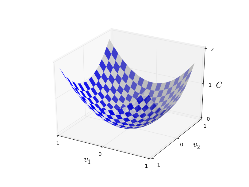
我们要找到 $C$ 的全局最小值。一种做法是计算函数的导数，找到各个极值。课本上的导数很好求解。不幸的是，现实生活中，问题所代表的函数经常包含过多的变量。尤其是神经网络中，有数以万计的权值和偏移，不可能直接求取极值。

幸好还有其他方法。让我们换种思维方式，对比那个函数图像，将函数看作一个山谷，并假设有一个小球沿着山谷斜坡滑动。直觉告诉我们小球最终会滑向坡底。也许这就能用来找到最小值？我们为“小球”随机选择一个起点，然后模拟“小球”沿斜坡滑动。“小球”运动的方向可以通过偏导数确定，这些偏导数包含了山谷形状的信息。

是否需要牛顿力学公式来获取小球的运动，考虑摩擦力和重力呢？并不需要，我们是在制定一个最小化 C 的算法，而不是去精确模拟物理学规律。

让我们记球在$ v_1 $ 方向移动了很小的量 $ \Delta v_1 $,在$ v_2 $ 方向移动了很小的量 $ \Delta v_2 $，总的 C 的改变量为：

$$ \Delta C \approx {\alpha C \over \alpha v_1 } \Delta v_1 + { \alpha C \over \alpha v_2 } \Delta v_2 $$

我们目标是找到一组 $\Delta v_1 $ 和 $\Delta v_2 $，使 $\Delta C $ 为负，即使球向谷底滚去。接下来记 $\Delta v \equiv (\Delta v_1, \Delta v_2)^T$ 为 $v$ 的总变化，并且记梯度向量 $\nabla C$ 为：

导数，偏导数，方向导数，梯度

$$ \nabla C \equiv \left( \frac{\partial C}{\partial v_1}, \frac{\partial C}{\partial v_2} \right)^T $$

其中梯度向量符号$\nabla C$会比较抽象，因为它纯粹就是一个数学上的概念。有了梯度符号，我们可以上面式子改写为

公式 4

$$\Delta C \approx \nabla C \cdot \Delta v$$

从该式可以看出，梯度向量$\nabla C$将 $v$ 的变化反应到 $C$ 中，且我们也找到了如何让$\Delta C$为负的方法。尤其是当我们选择

公式5

$$\Delta v = -\eta \nabla C$$

当 $η$ 是一个很小的正参数时（其实该参数就是学习率）,公式 4 表明 $ \Delta C \approx -\eta\nabla C \cdot \nabla C = -\eta |\nabla C|^2 $。因为 $| \nabla C|^2 \geq 0$ ,能保证 $\Delta C \leq 0$。这正是我们需要的特性！在梯度下降学习法中，我们使用公式 5 计算 $\Delta v$ ，然后移动球到新的位置：

公式6

$$ v \rightarrow v’ = v -\eta \nabla C $$

然后不停使用这一公式计算下一步，直到 $C$ 不再减小为止，即找到了全局最小值。

总结一下，首先重复计算梯度 $ \nabla C $，然后向相反方向移动，画成图就是

请注意，上述梯度下降的规则并没有复制出真正的物理运动。在真实生活中，球有动量，滚向谷底后还会继续滚上去，在摩擦力的作用下才会最终停下。但我们的算法中没这么复杂。

为了使算法正常工作，公式 4 中的学习率 $\eta$ 要尽可能的小，不然最终可能 $\Delta C > 0$。同时学习率不能过小，不然会导致每一次迭代中 $\Delta v$ 过小，算法工作会非常慢。

尽管到现在我们一直用两个变量的函数 $C$ 举例。但其实对于多变量的函数，这仍是适用的。假设 $C$ 有 $m$ 个变量，$v1,…,vm，$那么变化 $\Delta C$ 为

公式7

$$ \Delta C \approx \nabla C \cdot \Delta v $$

其中 $ \Delta v = (\Delta v_1,\ldots, \Delta v_m)^T $ ,梯度向量 $ \nabla C $ 为

公式8

$$ \nabla C \equiv \left(\frac{\partial C}{\partial v_1}, \ldots, \frac{\partial C}{\partial v_m}\right)^T $$

梯度下降法虽然简单，但实际上很有效，也是一个经典的最优化方法，在神经网络中我们将用它来寻找代价函数的最小值。

同时，人们研究了大量梯度下降法的变种，包括去模拟真实的物理学，但都效果不好。因为这些变种算法不光计算一次偏导数，还需要计算二次偏导，这对计算机来说是巨大的挑战，尤其是有着上百万神经元的神经网络。

我们将使用梯度下降法来来找到权重 $w_k$ 和偏移 $b_l$。类比上述的梯度法，这里变量 $v_j$ 即为权重和偏移，而梯度 $\nabla C$ 为 $\partial C / \partial w_k$ 和 $\partial C/ \partial b_l$。梯度下降的更新规则如下：

公式9

$$ w_k \rightarrow w_k’ = w_k-\eta \frac{\partial C}{\partial w_k}$$

公式10

$$ b_l \rightarrow b_l’ = b_l-\eta \frac{\partial C}{\partial b_l} $$

在适用梯度下降法时仍有一些挑战，比如公式 (1) 中代价函数是每一个训练样本的误差 $C_x \equiv \frac{|y(x)-a|^2}{2}$ 的平均值。这意味着计算梯度时，需要每一个训练样本计算梯度。当样本数量很多时，就会造成性能的问题。

随机梯度下降法能够解决这一问题，加速学习过程。算法每次随机从训练输入中选取 $m$ 个数据，$X_1,X_2…X_m$,记为 mini-batch。当 $m$ 足够大时，$\nabla C_{X_j}$ 将十分接近所有样本的平均值 $\nabla C_x$ 即：

公式11

$$\frac{\sum_{j=1}^m \nabla C_{X_{j}}}{m} \approx \frac{\sum_x \nabla C_x}{n} = \nabla C$$

交换等式两边得

公式12

$$\nabla C \approx \frac{1}{m} \sum_{j=1}^m \nabla C_{X_{j}}$$

这样，我们把总体的梯度转换成计算随机选取的 mini-batch 的梯度。将随机梯度下降法运用到神经网络中，则权重和偏移为

公式13

$$w_k \rightarrow w_k’ = w_k-\frac{\eta}{m} \sum_j \frac{\partial C_{X_j}}{\partial w_k}$$

公式14

$$b_l \rightarrow b_l’ = b_l-\frac{\eta}{m} \sum_j \frac{\partial C_{X_j}}{\partial b_l}$$

这里我要特别说明一下，每一个 $w$ 的改变，

其中，求和是对当前 mini-batch 中训练样本 $X_j$ 求和。然后选取下一组 mini-batch 重复上述过程，直到所有的训练输入全部选取完成，训练的一个 epoch 完成。

接着我们可以开始一个新的 epoch。

对于 MNIST 数据集来说，一共有 $n=60000$ 个数据，如果选择 mini-batch 的大小 $m=10$，则计算梯度的速度可以比原先快 6000 倍。当然，加速计算的结果只是近似值，尽管会有一些统计学上的波动，但精确的梯度计算并不重要，只要小球下降的大方向不错就行。为什么我敢这么说，因为实践证明了啊，随机梯度也是大多数自学习算法的基石。

前向传播代码

我们将官方的 MNIST 数据分成三部分，50000 个训练集，10000 个验证集，10000 个测试集。验证集用于在训练过程中实时观察神经网络正确率的变化，测试集用于测试最终神经网络的正确率。

下面介绍一下代码的核心部分。首先是 Network 类的初始化部分：

class Network(object):
    def __init__(self, sizes):
        self.num_layers = len(sizes)
        self.sizes = sizes
        self.biases = [np.random.randn(y, 1) for y in sizes[1:]]
        self.weights = [np.random.randn(y, x) 
                        for x, y in zip(sizes[:-1], sizes[1:])]

列表 sizes 表示神经网络每一层所包含的神经元个数。比如我们想创建一个 2 个输入神经元，3 个神经元在中间层，一个输出神经元的网络，那么可以

net = Network([2, 3, 1])

偏移和权重都是使用 np.random.randn 函数随机初始化的，平均值为 0，标准差为 1。这种随机初始化并不是最佳方案，后续文章会逐步优化。

请注意，偏移和权重被初始化为 Numpy 矩阵。net.weights[1] 代表连接第二和第三层神经元的权重。

下面是 sigmoid 函数的定义：

def sigmoid(z):
    return 1.0/(1.0+np.exp(-z))

注意到虽然输入 z 是向量，但 Numpy 能够自动处理，为向量中的每一个元素作相同的 sigmoid 运算。

然后是计算 sigmoid 函数的导数：

def sigmoid_prime(z):
    """Derivative of the sigmoid function."""
    return sigmoid(z)*(1-sigmoid(z))

每一层相对于前一层的输出为

$$a’ = \sigma(w a + b)$$

对应的是 feedforward 函数当：

def feedforward(self, a):
    """Return the output of the network if "a" is input."""
    for b, w in zip(self.biases, self.weights):
        a = sigmoid(np.dot(w, a)+b)
    return a

当然，Network 对象最重要的任务还是自学习。下面的 SGD 函数实现了随机梯度下降法：

def SGD(self, training_data, epochs, mini_batch_size, eta,
        test_data=None):
    """Train the neural network using mini-batch stochastic
    gradient descent.  The "training_data" is a list of tuples
    "(x, y)" representing the training inputs and the desired
    outputs.  The other non-optional parameters are
    self-explanatory.  If "test_data" is provided then the
    network will be evaluated against the test data after each
    epoch, and partial progress printed out.  This is useful for
    tracking progress, but slows things down substantially."""
    if test_data: n_test = len(test_data)
    n = len(training_data)
    for j in xrange(epochs):
        random.shuffle(training_data)
        mini_batches = [
            training_data[k:k+mini_batch_size]
            for k in xrange(0, n, mini_batch_size)]
        for mini_batch in mini_batches:
            self.update_mini_batch(mini_batch, eta)
        if test_data:
            print "Epoch {0}: {1} / {2}".format(
                j, self.evaluate(test_data), n_test)
        else:
            print "Epoch {0} complete".format(j)

列表 training_data 是由 (x,y) 元组构成，代表训练集的输入和期望输出。而 test_data 则是验证集（非测试集，这里变量名有些歧义），在每一个 epoch 结束时对神经网络正确率做一下检测。其他变量的含义比较显见，不再赘述。

SGD 函数在每一个 epoch 开始时随机打乱训练集，然后按照 mini-batch 的大小对数据分割。在每一步中对一个 mini_batch 计算梯度，在 self.update_mini_batch(mini_batch, eta) 更新权重和偏移：

def update_mini_batch(self, mini_batch, eta):
    """Update the network's weights and biases by applying
    gradient descent using backpropagation to a single mini batch.
    The "mini_batch" is a list of tuples "(x, y)", and "eta"
    is the learning rate."""
    nabla_b = [np.zeros(b.shape) for b in self.biases]
    nabla_w = [np.zeros(w.shape) for w in self.weights]
    for x, y in mini_batch:
        delta_nabla_b, delta_nabla_w = self.backprop(x, y)
        nabla_b = [nb+dnb for nb, dnb in zip(nabla_b, delta_nabla_b)]
        nabla_w = [nw+dnw for nw, dnw in zip(nabla_w, delta_nabla_w)]
    self.weights = [w-(eta/len(mini_batch))*nw 
                    for w, nw in zip(self.weights, nabla_w)]
    self.biases = [b-(eta/len(mini_batch))*nb 
                   for b, nb in zip(self.biases, nabla_b)]

其中最关键的是

delta_nabla_b, delta_nabla_w = self.backprop(x, y)

这就是反向转播算法，这是一个快速计算代价函数梯度的方法。所以 update_mini_batch 仅仅是计算这些梯度，然后用来更新 self.weights 和 self.biases。

反向传播

首先是明确的权重定义。使用 $w^l_{jk}$ 表示权重，代表连接 $(l-1)^{\rm th}$ 层第 $k^{\rm th}$ 个神经元 和 $l^{\rm th}$ 层第 $j^{\rm th}$ 个神经元的权重。举例来说，第二层第四个神经元和第三层第二个神经元之间的权重连接为

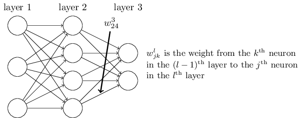
对于网络的偏移和激励我们将使用类似的符号。即 $b^l_j$ 是 $l^{\rm th}$ 层第 $j^{\rm th}$ 个神经元的偏移，$a^l_j$ 是 $l^{\rm th}$ 层第 $j^{\rm th}$ 个神经元的激励。如图所示：

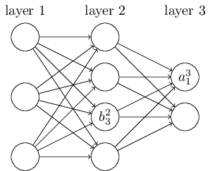
有了这些记号，第 $l^{\rm th}$ 层第 $ j^{\rm th} $ 个神经元的激励 $ a^l_j $可以由第 $(l-1)^{\rm th}$ 层的所有激励求得：

公式15

$$a^{l}j = \sigma\left( \sum_k w^{l}{jk} a^{l-1}_k + b^l_j \right)$$

其中，求和是对第 $(l-1)^{\rm th}$ 层所有的神经元求和。为了将表达式转换成矩阵的形式，这里为每一层 $l$ 定义一个权重矩阵 $w^l$。该矩阵中第 $j^{\rm th}$ 行第 $k^{\rm th}$ 列的元素为 $w^l_{jk}$。类似的，为每一层定义了一个偏移向量 $b^l$，每一个神经元的偏移为 $b^l_j$。最后，我们定义第 $k$ 层所有的激励 $a^l_j$ 的集合为激励向量 $a^l$。

对于公式 15，我们还需要向量化函数 $σ$。因为我们不是将整个矩阵作为一个参数传递给函数，而是对矩阵的每一个元素应用相同的函数，即 $\sigma(v)$ 的元素为 $\sigma(v)_j = \sigma(v_j)$。举例来说，假如我们有一个函数 $f(x)=x^2$，那么函数 $f$ 的向量化是：

公式16

$$f\left(\left[ \begin{array}{c} 2 \ 3 \end{array} \right] \right) = \left[ \begin{array}{c} f(2) \ f(3) \end{array} \right] = \left[ \begin{array}{c} 4 \ 9 \end{array} \right]$$

有了这些，我们将公式 15 重写成下列更紧凑的形式：

公式17

$$a^{l} = \sigma(w^l a^{l-1}+b^l)$$

这个表达式给了我们更全局的视角：本层的激励是如何与上一层的激励相关联的。计算$a^l$,会计算出中间结构 $z^l \equiv w^l a^{l-1}+b^l$。这一项我们称之为第 $l$ 层的加权输入。

$z^l$的每一个元素为 $z^l_j= \sum_k w^l_{jk} a^{l-1}_k+b^l_j$ ,即 $z^l_j$ 是第 $l$ 层第 $j$ 个神经元激励函数的加权输入。公式 17 有时也会写作 $a^l =\sigma(z^l)$。

代价函数的两个前提假设

反向传播算法是为了计算代价函数 $C$ 的两个偏导数 $\partial C / \partial w$ 和 $\partial C / \partial b$。

首先看我们的二次代价函数

公式18

$$ C = \frac{1}{2n} \sum_x |y(x)-a^L(x)|^2 $$

其中 $n$ 是训练数据的总数，求和是对每一个数据求和，$y=y(x)$ 是相应的期望输出，$L$ 是网络的总层数，$a^L = a^L(x)$ 是实际的网络输出。

第一个假设是代价函数可以写作时单个训练数据误差 $C_x =\frac{1}{2} |y-a^L |^2$ 的平均值 $C = \frac{1}{n} \sum_x C_x$。这个假设对于后续介绍的其他代价函数也是成立的。

之所以这么假设是因为反向传播算法只能够计算单个训练数据的偏导数 $\partial C_x / \partial w$ 和 $\partial C_x / \partial b$。最后对所有数据求平均值得 $\partial C / \partial w$ 和 $\partial C / \partial b$。

第二个假设是误差可以写作神经网络输出的函数：

例如，二次代价函数就满足这一要求，单个训练数据 $x$ 的二次误差可以写成：

公式19

$$C = \frac{1}{2} |y-a^L|^2 = \frac{1}{2} \sum_j (y_j-a^L_j)^2$$

其中，对单个样本来说，$x$ 是定值，期望输出 $y$ 也是定值，唯一的变量就是网络输出 $a^L$，即满足第二条假设。

反向传播的四个基本公式

反向传播算法基于最基本的线性代数操作，比如向量相加、向量与矩阵相乘等。其中有一个比较少见，假设 $s$ 和 $t$ 是两个同维的向量，我们定义 $s \odot t$为两个向量对应分量的乘积。那么其每个元素为 $(s \odot t)_j = s_jt_j$。例如，

公式20

$$\left[\begin{array}{c} 1 \ 2 \end{array}\right] \odot \left[\begin{array}{c} 3 \ 4\end{array} \right] = \left[ \begin{array}{c} 1 \times 3 \ 2 \times 4 \end{array} \right] = \left[ \begin{array}{c} 3 \ 8 \end{array} \right]$$

这种元素对元素的乘积也称作 Hadamard 积或者是 Schur 积。Numpy 对这种运算有着良好的优化。

然后我们继续引入一个中间变量 $\delta^l_j$，我们称作第 $l$ 层第 $j$ 个神经元的误差。为了形象地理解误差到底是什么，假设在我们的神经网络中有一个小妖精：

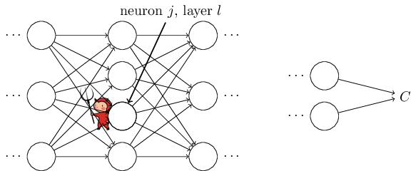
这个妖精坐在 $l$ 层的第 $j$ 个神经元上。当输入到来时，它故意扰乱神经元的正常工作。它在神经元的加权输入中加入了一个小的变化 $\Delta z^l_j$，这样输出变成了 $\sigma(z^l_j+\Delta z^l_j)$。这个变化向后层神经网络传递，最终到输出层导致误差相应地改变为 $\frac{\partial C}{\partial z^l_j} \Delta z^l_j$。

现在，我们钦定了这个妖精是个好妖精，在试图帮助我们减小误差。当 $\frac{\partial C}{\partial z^l_j}$ 是个很大的正数（负数）时，通过选择 $\Delta z^l_j$ 为负值（正）即可减小误差。但如果 $\frac{\partial C}{\partial z^l_j}$ 接近于零，那么这时这个好妖精无论做什么都对误差结果影响不大，这时可以认为网络接近最优值。

以上说明 $\frac{\partial C}{\partial z^l_j}$是一个可以用来量化神经元误差 的量。所以我们定义

公式21

$$\delta^l_j \equiv \frac{\partial C}{\partial z^l_j}$$

你可能会奇怪为什么要引入一个新的中间量–加权输入 $z^l_j$，而不是直接使用激励 $a^l_j$ ？纯粹是因为这个中间量让最后的反向传播表达式更简洁。

输出层的误差，$\delta^L$ ，该误差分量由下式给出

公式BP1

$$ \delta^L_j = \frac{\partial C}{\partial a^L_j} \sigma’(z^L_j) $$

这是一个非常自然的表达式，等式右边第一项为 $\partial C / \partial a^L_j$，反映了误差在第 $j$ 个输出激励影响下变化的速度。若某个特定的输出神经元对误差 $C$ 影响不大，则 $\delta^L_j$ 很小。右边第二项为$\sigma’(z^L_j)$，反应了 $z^L_j$ 对激励函数 $\delta$ 的影响。

公式 (BP1) 非常容易计算。加权输入在 feedforward 正向传播时即可顺便计算，而 sigmoid 激励函数和二次代价函数的偏导也易可得。鉴于 (BP1) 是以每个元素的形式给出的，有必要改写成矩阵的形式：

公式BP1a

$$\delta^L = \nabla_a C \odot \sigma’(z^L)$$

这里，$\nabla_a C$ 是偏导数 $\partial C / \partial a^L_j$ 组成的向量。你可以认为 $\nabla_a C$ 反映了误差相对于输出激励的变化。由二次代价函数 $C = \frac{1}{2} \sum_j (y_j-a_j)^2$ 的偏导数 $\partial C / \partial a^L_j = (a_j-y_j)$ 可得：$\nabla_a C =(a^L-y)$。最终公式 (BP1) 变成

公式22

$$\delta^L = (a^L-y) \odot \sigma’(z^L)$$

通过下一层误差可以求本层误差，即

公式 BP2

$$\delta^l = ((w^{l+1})^T \delta^{l+1}) \odot \sigma’(z^l)$$

初看上去这个公式有点复杂，但其意义显而易见。$l+1$ 层的误差 $\delta^{l+1}$，通过权重矩阵的转置 $(w^{l+1})^T$ 反向转播到第 $l$ 层，然后与 $\sigma’(z^l)$ 做 Hadamard 积即可求得 $l$ 层的误差。

BP2的证明

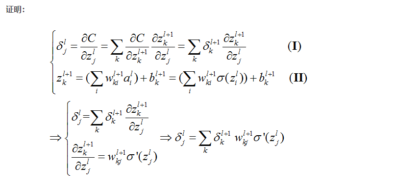
证明解释

首先看（I）式，$ \delta^l_j = \frac{\partial C}{\partial Z^l_j} $,就是误差（error）的定义，这个简单。
通过公式 (BP1) 和公式 (BP2) 的组合，每一层的误差都能求得。

这个就是链式法则啦，我们知道前一层的输出可以作为后一层的输入，也就是说，可以认为前一层的$z$算式后一层$z$的变量（别晕）。应用复合函数链式法则，就能够得到这个式子了。

$\alpha C\over \alpha z_k^{l + 1}$相当于 $l+1$ 层的误差啦，所以可以简化为 $\delta_k^{l + 1}$。

再来看（II）式，这个公式就是计算$z$的，更加简单。不解释了。然后（II）式求偏导之后得到 $w_{kj}^{l+1} \delta’(z_j^l)$ 代入（I）的最终结果，就得到上面的结果了

BP2是上面这个式子的向量形式。

理解

通过这个公式，只要我知道l+1层的误差，那么我就能够知道l层的误差，由此，我就能够倒退直到第1层的误差。

这个式子就体现了误差的反向传播的特点。

然后BP1和BP2结合起来，我们就能够求出神经网络中任何一层，任何一个神经元上面的误差。

误差相对于偏移的变化率，即偏导数为

公式BP3

$$\frac{\partial C}{\partial b^l_j} = \delta^l_j$$

这意味着其偏导数就是误差的值本身，我们也可以简写为

公式23

$$\frac{\partial C}{\partial b} = \delta$$

误差相对于权重的变化率，即偏导数为

公式BP4

$$\frac{\partial C}{\partial w^l_{jk}} = a^{l-1}_k \delta^l_j$$

这意味着我们可以通过上一层的激励和本层的误差来求取偏导数，我们也可以简写为

公式24

$$\frac{\partial C}{\partial w} = a_{\rm in} \delta_{\rm out}$$

上一层的激励如果接近于零，$a_{\rm in} \approx 0$，那么 $\partial C / \partial w$ 也会非常小，这种情况下，权重的自学习速度减慢了。

反向传播算法

由公式 (BP1)-(BP4) 即可得反向传播算法的步骤如下：

首先，输入一个 mini-batch 量的训练数据。

然后，对每一个训练数据 $x$ 施加以下步骤：

正向传播：对每一层 $l=2,3,…,L$ 计算 $z^{x,l} = w^l a^{x,l-1}+b^l$ 和 $a^{x,l} = \sigma(z^{x,l})$。

计算最后一层误差 $\delta^{x,L}$ ：计算向量 $\delta^{x,L} = \nabla_a C_x \odot \sigma’(z^{x,L})$。

反向传播误差：对每一层 $l=L−1,L−2,…,2$ 计算 $\delta^{x,l} = ((w^{l+1})^T \delta^{x,l+1})\odot \sigma’(z^{x,l})$。

最后，为这个 mini-batch 中的训练数据计算下降的梯度：对于每一层 $l=L,L−1,…,2$ 更新权重和偏移 $w^l \rightarrow w^l-\frac{\eta}{m} \sum_x \delta^{x,l} (a^{x,l-1})^T, b^l \rightarrow b^l-\frac{\eta}{m}\sum_x \delta^{x,l}$。

写成代码即为

def backprop(self, x, y):
     """Return a tuple "(nabla_b, nabla_w)" representing the
     gradient for the cost function C_x.  "nabla_b" and
     "nabla_w" are layer-by-layer lists of numpy arrays, similar
     to "self.biases" and "self.weights"."""
     nabla_b = [np.zeros(b.shape) for b in self.biases]
     nabla_w = [np.zeros(w.shape) for w in self.weights]
     # feedforward
     activation = x
     activations = [x] # list to store all the activations, layer by layer
     zs = [] # list to store all the z vectors, layer by layer
     for b, w in zip(self.biases, self.weights):
         z = np.dot(w, activation)+b
         zs.append(z)
         activation = sigmoid(z)
         activations.append(activation)
     # backward pass
     delta = self.cost_derivative(activations[-1], y) * \
         sigmoid_prime(zs[-1])
     nabla_b[-1] = delta
     nabla_w[-1] = np.dot(delta, activations[-2].transpose())
     # Note that the variable l in the loop below is used a little
     # differently to the notation in Chapter 2 of the book.  Here,
     # l = 1 means the last layer of neurons, l = 2 is the
     # second-last layer, and so on.  It's a renumbering of the
     # scheme in the book, used here to take advantage of the fact
     # that Python can use negative indices in lists.
     for l in xrange(2, self.num_layers):
         z = zs[-l]
         sp = sigmoid_prime(z)
         delta = np.dot(self.weights[-l+1].transpose(), delta) * sp
         nabla_b[-l] = delta
         nabla_w[-l] = np.dot(delta, activations[-l-1].transpose())
     return (nabla_b, nabla_w)

完整代码

#### Libraries
# Standard library
import random

# Third-party libraries
import numpy as np

class Network(object):

    def __init__(self, sizes):
        """The list ``sizes`` contains the number of neurons in the
        respective layers of the network.  For example, if the list
        was [2, 3, 1] then it would be a three-layer network, with the
        first layer containing 2 neurons, the second layer 3 neurons,
        and the third layer 1 neuron.  The biases and weights for the
        network are initialized randomly, using a Gaussian
        distribution with mean 0, and variance 1.  Note that the first
        layer is assumed to be an input layer, and by convention we
        won't set any biases for those neurons, since biases are only
        ever used in computing the outputs from later layers."""
        self.num_layers = len(sizes)
        self.sizes = sizes
        self.biases = [np.random.randn(y, 1) for y in sizes[1:]]
        self.weights = [np.random.randn(y, x)
                        for x, y in zip(sizes[:-1], sizes[1:])]

    def feedforward(self, a):
        """Return the output of the network if ``a`` is input."""
        for b, w in zip(self.biases, self.weights):
            a = sigmoid(np.dot(w, a)+b)
        return a

    def SGD(self, training_data, epochs, mini_batch_size, eta,
            test_data=None):
        """Train the neural network using mini-batch stochastic
        gradient descent.  The ``training_data`` is a list of tuples
        ``(x, y)`` representing the training inputs and the desired
        outputs.  The other non-optional parameters are
        self-explanatory.  If ``test_data`` is provided then the
        network will be evaluated against the test data after each
        epoch, and partial progress printed out.  This is useful for
        tracking progress, but slows things down substantially."""
        if test_data: n_test = len(test_data)
        n = len(training_data)
        for j in xrange(epochs):
            random.shuffle(training_data)
            mini_batches = [
                training_data[k:k+mini_batch_size]
                for k in xrange(0, n, mini_batch_size)]
            for mini_batch in mini_batches:
                self.update_mini_batch(mini_batch, eta)
            if test_data:
                print "Epoch {0}: {1} / {2}".format(
                    j, self.evaluate(test_data), n_test)
            else:
                print "Epoch {0} complete".format(j)

    def update_mini_batch(self, mini_batch, eta):
        """Update the network's weights and biases by applying
        gradient descent using backpropagation to a single mini batch.
        The ``mini_batch`` is a list of tuples ``(x, y)``, and ``eta``
        is the learning rate."""
        nabla_b = [np.zeros(b.shape) for b in self.biases]
        nabla_w = [np.zeros(w.shape) for w in self.weights]
        for x, y in mini_batch:
            delta_nabla_b, delta_nabla_w = self.backprop(x, y)
            nabla_b = [nb+dnb for nb, dnb in zip(nabla_b, delta_nabla_b)]
            nabla_w = [nw+dnw for nw, dnw in zip(nabla_w, delta_nabla_w)]
        self.weights = [w-(eta/len(mini_batch))*nw
                        for w, nw in zip(self.weights, nabla_w)]
        self.biases = [b-(eta/len(mini_batch))*nb
                       for b, nb in zip(self.biases, nabla_b)]

    def backprop(self, x, y):
        """Return a tuple ``(nabla_b, nabla_w)`` representing the
        gradient for the cost function C_x.  ``nabla_b`` and
        ``nabla_w`` are layer-by-layer lists of numpy arrays, similar
        to ``self.biases`` and ``self.weights``."""
        nabla_b = [np.zeros(b.shape) for b in self.biases]
        nabla_w = [np.zeros(w.shape) for w in self.weights]
        # feedforward
        activation = x
        activations = [x] # list to store all the activations, layer by layer
        zs = [] # list to store all the z vectors, layer by layer
        for b, w in zip(self.biases, self.weights):
            z = np.dot(w, activation)+b
            zs.append(z)
            activation = sigmoid(z)
            activations.append(activation)
        # backward pass
        delta = self.cost_derivative(activations[-1], y) * \
            sigmoid_prime(zs[-1])
        nabla_b[-1] = delta
        nabla_w[-1] = np.dot(delta, activations[-2].transpose())
        # Note that the variable l in the loop below is used a little
        # differently to the notation in Chapter 2 of the book.  Here,
        # l = 1 means the last layer of neurons, l = 2 is the
        # second-last layer, and so on.  It's a renumbering of the
        # scheme in the book, used here to take advantage of the fact
        # that Python can use negative indices in lists.
        for l in xrange(2, self.num_layers):
            z = zs[-l]
            sp = sigmoid_prime(z)
            delta = np.dot(self.weights[-l+1].transpose(), delta) * sp
            nabla_b[-l] = delta
            nabla_w[-l] = np.dot(delta, activations[-l-1].transpose())
        return (nabla_b, nabla_w)

    def evaluate(self, test_data):
        """Return the number of test inputs for which the neural
        network outputs the correct result. Note that the neural
        network's output is assumed to be the index of whichever
        neuron in the final layer has the highest activation."""
        test_results = [(np.argmax(self.feedforward(x)), y)
                        for (x, y) in test_data]
        return sum(int(x == y) for (x, y) in test_results)

    def cost_derivative(self, output_activations, y):
        """Return the vector of partial derivatives \partial C_x /
        \partial a for the output activations."""
        return (output_activations-y)

#### Miscellaneous functions
def sigmoid(z):
    """The sigmoid function."""
    return 1.0/(1.0+np.exp(-z))

def sigmoid_prime(z):
    """Derivative of the sigmoid function."""
    return sigmoid(z)*(1-sigmoid(z))