这是 pytorch 中和 CNN 有关的方法。
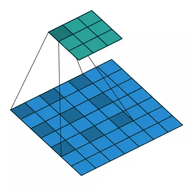
卷积
nn.Conv2d
在这里还是建议看官方文档。
torch.nn.Conv2d(in_channels, out_channels, kernel_size, stride=1, padding=0, dilation=1, groups=1, bias=True, padding_mode=’zeros’)
官网文档上有很多很有帮助的公式,在这里就不贴了。
Parameters
in_channels (int) – 输入图像通道数out_channels (int) – 卷积产生的通道数kernel_size (int or tuple) – 卷积核尺寸,可以设为1个int型数或者一个(int, int)型的元组。例如(2,3)是高2宽3卷积核stride (int or tuple, optional) – 卷积步长,默认为1。可以设为1个int型数或者一个(int, int)型的元组。padding (int or tuple, optional) – 填充操作,控制padding_mode的数目。padding_mode (string, optional) – padding模式,默认为Zero-padding 。dilation (int or tuple, optional) – 扩张操作:控制kernel点(卷积核点)的间距,默认值:1。groups (int, optional) – group参数的作用是控制分组卷积,默认不分组,为1组。bias (bool, optional) – 为真,则在输出中添加一个可学习的偏差。默认:True。
padding mode
- zeros
- reflect
- replicate
- circular
关于这个,你可以参考我下面两个博文,但是, nn.Conv2d 里面的填充方式,和下面写的 torch | 填充方式,好像有区别,但是,我没验证。
dilation
扩张卷积(也叫空洞卷积)
dilation 操作动图演示如下:
- Dilated Convolution with a 3 x 3 kernel and dilation rate 2 扩张卷积核为3×3,扩张率为2
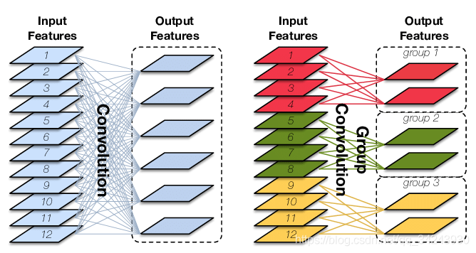
参数groups——分组卷积
Group Convolution顾名思义,则是对输入feature map进行分组,然后每组分别卷积。
假设输入feature map的尺寸仍为C ∗ H ∗ W,输出feature map的数量为N个,如果设定要分成G个groups,则每组的输入feature map数量为 $\frac{C}{G}$ ,每组的输出feature map数量为 $ \frac{N}{G} $。每个卷积核的尺寸为 $ \frac{C}{G} * K * K $,卷积核的总数仍为N ,每组的卷积核数量为 $ \frac{N}{G} $,卷积核只与其同组的输入map进行卷积,卷积核的总参数量为 $ N * \frac{C}{G} * K * K $,可见,总参数量减少为原来的 $ \frac{1}{G} $,其连接方式如下图右所示,group1输出map数为2,有2个卷积核,每个卷积核的channel数为4,与group1的输入map的channel数相同,卷积核只与同组的输入map卷积,而不与其他组的输入map卷积。
代码例子
案例一
1
2
3
4
5
6
7
| conv = nn.Conv2d(1, 1, kernel_size=(1, 1), stride=(1, 1), padding=(1, 2), bias=False)
init.constant(conv.weight, 2)
print(conv.weight)
input = torch.tensor([[[[1., 1.], [2., 2.]]]])
print(input)
print(conv(input))
|
输出
1
2
3
4
5
6
7
| tensor([[[[2.]]]], requires_grad=True)
tensor([[[[1., 1.],
[2., 2.]]]])
tensor([[[[0., 0., 0., 0., 0., 0.],
[0., 0., 2., 2., 0., 0.],
[0., 0., 4., 4., 0., 0.],
[0., 0., 0., 0., 0., 0.]]]], grad_fn=<MkldnnConvolutionBackward>)
|
案例二
1
2
3
4
5
6
7
| conv = nn.Conv2d(1, 1, kernel_size=(1, 1), stride=(1, 1), padding=(2, 1), bias=False)
init.constant(conv.weight, 2)
print(conv.weight)
input = torch.tensor([[[[1., 1.], [2., 2.]]]])
print(input)
print(conv(input))
|
输出
1
2
3
4
5
6
7
8
9
| tensor([[[[2.]]]], requires_grad=True)
tensor([[[[1., 1.],
[2., 2.]]]])
tensor([[[[0., 0., 0., 0.],
[0., 0., 0., 0.],
[0., 2., 2., 0.],
[0., 4., 4., 0.],
[0., 0., 0., 0.],
[0., 0., 0., 0.]]]], grad_fn=<MkldnnConvolutionBackward>)
|
案例三
1
2
3
4
5
6
7
| conv = nn.Conv2d(1, 1, kernel_size=(1, 1), stride=(1, 2), padding=(2, 1), bias=False)
init.constant(conv.weight, 2)
print(conv.weight)
input = torch.tensor([[[[1., 1.], [2., 2.]]]])
print(input)
print(conv(input))
|
输出
1
2
3
4
5
6
7
8
9
| tensor(, requires_grad=True)
tensor(
)
tensor(
, grad_fn=<MkldnnConvolutionBackward>)
|
nn.ConvTranspose2d
pytorch 的 nn.ConvTranspose2d 和 nn.Conv2d 的 padding 是相反的,一个是向内扩充,一个是向外扩充。
案例一
1
2
3
4
5
6
7
8
9
10
11
12
| dconv = nn.ConvTranspose2d(in_channels=1, out_channels=1,
kernel_size=(1, 1),
stride=1,
padding=0,
output_padding=(0, 0),
bias=False)
init.constant_(dconv.weight, 2)
print(dconv.weight)
input = torch.tensor([[[[1., 1., 1.], [2., 2., 2.], [3., 3., 3.]]]])
print(input)
print(dconv(input))
|
输出
1
2
3
4
5
6
7
| tensor([[[[2.]]]], requires_grad=True)
tensor([[[[1., 1., 1.],
[2., 2., 2.],
[3., 3., 3.]]]])
tensor([[[[2., 2., 2.],
[4., 4., 4.],
[6., 6., 6.]]]], grad_fn=<SlowConvTranspose2DBackward>)
|
解析
首先,原数据是
1
2
3
| 1 , 1 , 1
2 , 2 , 2
3 , 3 , 3
|
然后 stride = 1 表示,这个矩阵不需要扩充。
计算出来结果后
1
2
3
| 2 , 2 , 2
4 , 4 , 4
6 , 6 , 6
|
padding = 0,表示不向内扩充,最后数据最后变成
1
2
3
| 2 , 2 , 2
4 , 4 , 4
6 , 6 , 6
|
案例二
代码如下
1
2
3
4
5
6
7
8
9
10
11
12
| dconv = nn.ConvTranspose2d(in_channels=1, out_channels=1,
kernel_size=(1, 1),
stride=1,
padding=1,
output_padding=(0, 0),
bias=False)
init.constant_(dconv.weight, 2)
print(dconv.weight)
input = torch.tensor([[[[1., 1., 1.], [2., 2., 2.], [3., 3., 3.]]]])
print(input)
print(dconv(input))
|
输出
1
2
3
4
5
| tensor([[[[2.]]]], requires_grad=True)
tensor([[[[1., 1., 1.],
[2., 2., 2.],
[3., 3., 3.]]]])
tensor([[[[4.]]]], grad_fn=<SlowConvTranspose2DBackward>)
|
原数据为
1
2
3
| 1 , 1 , 1
2 , 2 , 2
3 , 3 , 3
|
经过和 weight 相乘,变成
1
2
3
| 2 , 2 , 2
4 , 4 , 4
6 , 6 , 6
|
padding 向内压缩 1,最后变成
案例三
代码如下
1
2
3
4
5
6
7
8
9
10
11
12
| dconv = nn.ConvTranspose2d(in_channels=1, out_channels=1,
kernel_size=(1, 1),
stride=2,
padding=0,
output_padding=(0, 0),
bias=False)
init.constant_(dconv.weight, 2)
print(dconv.weight)
input = torch.tensor([[[[1., 1., 1.], [2., 2., 2.], [3., 3., 3.]]]])
print(input)
print(dconv(input))
|
输出
1
2
3
4
5
6
7
8
9
| tensor([[[[2.]]]], requires_grad=True)
tensor([[[[1., 1., 1.],
[2., 2., 2.],
[3., 3., 3.]]]])
tensor([[[[2., 0., 2., 0., 2.],
[0., 0., 0., 0., 0.],
[4., 0., 4., 0., 4.],
[0., 0., 0., 0., 0.],
[6., 0., 6., 0., 6.]]]], grad_fn=<SlowConvTranspose2DBackward>)
|
解析,其中原数据为
1
2
3
| 1 , 1 , 1
2 , 2 , 2
3 , 3 , 3
|
因为 stride = 2,所以,数据会进行扩充,变成
1
2
3
4
5
| 1 , 0 , 1 , 0 , 1
0 , 0 , 0 , 0 , 0
2 , 0 , 2 , 0 , 2
0 , 0 , 0 , 0 , 0
3 , 0 , 3 , 0 , 3
|
后面。。。
案例四
代码如下
1
2
3
4
5
6
7
8
9
10
11
12
| dconv = nn.ConvTranspose2d(in_channels=1, out_channels=1,
kernel_size=(1, 1),
stride=2,
padding=1,
output_padding=(0, 0),
bias=False)
init.constant_(dconv.weight, 2)
print(dconv.weight)
input = torch.tensor([[[[1., 1., 1.], [2., 2., 2.], [3., 3., 3.]]]])
print(input)
print(dconv(input))
|
输出
1
2
3
4
5
6
7
| tensor([[[[2.]]]], requires_grad=True)
tensor([[[[1., 1., 1.],
[2., 2., 2.],
[3., 3., 3.]]]])
tensor([[[[0., 0., 0.],
[0., 4., 0.],
[0., 0., 0.]]]], grad_fn=<SlowConvTranspose2DBackward>)
|
解析,其中原数据为
1
2
3
| 1 , 1 , 1
2 , 2 , 2
3 , 3 , 3
|
因为 stride = 2,所以,数据会进行扩充,变成
1
2
3
4
5
| 1 , 0 , 1 , 0 , 1
0 , 0 , 0 , 0 , 0
2 , 0 , 2 , 0 , 2
0 , 0 , 0 , 0 , 0
3 , 0 , 3 , 0 , 3
|
接着,和 weight 做计算,变成
1
2
3
4
5
| 2 , 0 , 2 , 0 , 2
0 , 0 , 0 , 0 , 0
4 , 0 , 4 , 0 , 4
0 , 0 , 0 , 0 , 0
6 , 0 , 6 , 0 , 6
|
又因为 padding = 1 ,所以,内压缩 1「上下左右各删除1行或者1列」,最终数据变成为
1
2
3
| 0 , 0 , 0
0 , 4 , 0
0 , 0 , 0
|
案例五
根据案例四我们来讲一下 output_padding。
先说结论,out_padding 会向输出数据的右侧和下侧添加数据,直接看代码。
加下列
1
2
3
4
5
6
7
8
9
10
11
12
| dconv = nn.ConvTranspose2d(in_channels=1, out_channels=1,
kernel_size=(1, 1),
stride=2,
padding=1,
output_padding=(0, 1),
bias=False)
init.constant_(dconv.weight, 2)
print(dconv.weight)
input = torch.tensor([[[[1., 1., 1.], [2., 2., 2.], [3., 3., 3.]]]])
print(input)
print(dconv(input))
|
输出
1
2
3
4
5
6
7
| tensor([[[[2.]]]], requires_grad=True)
tensor([[[[1., 1., 1.],
[2., 2., 2.],
[3., 3., 3.]]]])
tensor([[[[0., 0., 0., 0.],
[0., 4., 0., 4.],
[0., 0., 0., 0.]]]], grad_fn=<SlowConvTranspose2DBackward>)
|
加右列
1
2
3
4
5
6
7
8
9
10
11
12
| dconv = nn.ConvTranspose2d(in_channels=1, out_channels=1,
kernel_size=(1, 1),
stride=2,
padding=1,
output_padding=(1, 0),
bias=False)
init.constant_(dconv.weight, 2)
print(dconv.weight)
input = torch.tensor([[[[1., 1., 1.], [2., 2., 2.], [3., 3., 3.]]]])
print(input)
print(dconv(input))
|
输出
1
2
3
4
5
6
7
8
| tensor([[[[2.]]]], requires_grad=True)
tensor([[[[1., 1., 1.],
[2., 2., 2.],
[3., 3., 3.]]]])
tensor([[[[0., 0., 0.],
[0., 4., 0.],
[0., 0., 0.],
[0., 6., 0.]]]], grad_fn=<SlowConvTranspose2DBackward>)
|
案例六
当,卷积核不是常数,而是矩阵的时候。
代码如下
1
2
3
4
5
6
7
8
9
10
11
12
| dconv = nn.ConvTranspose2d(in_channels=1, out_channels=1,
kernel_size=(2, 3),
stride=2,
padding=0,
output_padding=(0, 0),
bias=False)
init.constant_(dconv.weight, 2)
print(dconv.weight)
input = torch.tensor([[[[1., 1., 1.]]]])
print(input)
print(dconv(input))
|
输出
1
2
3
4
5
6
| tensor([[[[2., 2., 2.],
[2., 2., 2.]]]], requires_grad=True)
tensor([[[[1., 1., 1.]]]])
tensor([[[[2., 2., 4., 2., 4., 2., 2.],
[2., 2., 4., 2., 4., 2., 2.]]]],
grad_fn=<SlowConvTranspose2DBackward>)
|
首先看一份动图
在这个动图里,我们要注意两点
比如,我输入为 2,卷积核为
那么,会拿着输入 2 乘以卷积核得到
比如,输入
卷积核为
整个计算流程是
1
2
3
|
2 * [ 2 , 2] = [4 , 4] 另外一侧 1 * [2 , 2] = [2 , 2]
[ 2 , 2] [4 , 4] [2 , 2] [2 , 2]
|
然后计算出的结果,我们会有一个相加的过程,也就是如动图所示,所以,最后的结果是
了解了上面的全部信息后,我们再来计算一下上面的代码过程。
原始数据为
经过 stride = 2 的扩充后,变成了
然后,卷积核计算再相加,就会变成
1
2
| 2., 2., 4., 2., 4., 2., 2.
2., 2., 4., 2., 4., 2., 2.
|
你可以自己计算一下。
案例七
我们不对图进行扩充
1
2
3
4
5
6
7
8
9
10
11
12
| dconv = nn.ConvTranspose2d(in_channels=1, out_channels=1,
kernel_size=(2, 3),
stride=1,
padding=0,
output_padding=(0, 0),
bias=False)
init.constant_(dconv.weight, 2)
print(dconv.weight)
input = torch.tensor([[[[1., 1., 1.]]]])
print(input)
print(dconv(input))
|
最后输出为
1
2
3
4
5
| tensor([[[[2., 2., 2.],
[2., 2., 2.]]]], requires_grad=True)
tensor([[[[1., 1., 1.]]]])
tensor([[[[2., 4., 6., 4., 2.],
[2., 4., 6., 4., 2.]]]], grad_fn=<SlowConvTranspose2DBackward>)
|
这个可以自己计算一下。
案例八
现在有一个终极问题,是 padding 是卷积生成之前,还是卷积生成之后,先说结论,是卷积生成之后,直接看代码。
1
2
3
4
5
6
7
8
9
10
11
12
| dconv = nn.ConvTranspose2d(in_channels=1, out_channels=1,
kernel_size=(2, 3),
stride=1,
padding=1,
output_padding=(0, 0),
bias=False)
init.constant_(dconv.weight, 2)
print(dconv.weight)
input = torch.tensor([[[[1., 1., 1.], [2., 2., 2.], [3., 3., 3.]]]])
print(input)
print(dconv(input))
|
输出
1
2
3
4
5
6
7
| tensor([[[[2., 2., 2.],
[2., 2., 2.]]]], requires_grad=True)
tensor([[[[1., 1., 1.],
[2., 2., 2.],
[3., 3., 3.]]]])
tensor([[[[12., 18., 12.],
[20., 30., 20.]]]], grad_fn=<SlowConvTranspose2DBackward>)
|
我来解释一下所有的计算过程。
首先原数据是
1
2
3
| 1 , 1 , 1
2 , 2 , 2
3 , 3 , 3
|
没有进行填充,然后和 weight 进行计算,根据动图上的计算表示,最后计算结果为「事实上,下面的计算结果,我并没有真的算出来,但是,大差不差,你们可以计算一下」
1
2
3
4
| 2 , 4 , 6 , 4 , 2
6 , 12 , 18 , 12 , 6
10 , 20 , 30 , 20 , 10
8 , 16 , 24 , 16 , 8
|
然后 padding=1,我们减去上下左右,变成
1
2
| 12 , 18 , 12
20 , 30 , 20
|
池化
优化
nn.BatchNorm2d